DCA - A Theoretical Approach
Very often, I see investors, retail investors and institutonal ones, talk about DCA (Dollar Cost Averaging), asserting that it would be a preferred way to invest on volatile assets (e.g. cryptocurrencies). However, on the other hand, some studies pretend that DCA is not optimal compared to lump sum.
The goal of this post is to propose a very simple, yet powerful model of what a DCA could be from a quantitative point of view, and see to what extent the statement “DCA is suboptimal” is true.
The model
DCA, at its core principle, is simply taking a fixed amount of money (consider a position you would be interested in), and instead of entering all at once, we instead spread our entry point accross $n$ evenly spaced ones.
In our model, we will assume that there is a time $t_0$ at which we have an estimate of the first two moments of the probability distribution of returns. To simplify, we will consider a 1D case, since most mean-variance model can be locally diagnoalized. We will denote by $\mu$ the expectation of returns, and $\sigma$ their standard deviation.
We will denote $t_1, …, t_n$ the moments at which we enter a new fraction of the position. We have for all $i$, $T_i := t_i - t_{i-1}$. For simplicity, and because most computational model eventually enforce tackling te discrete case ($T := T_1 + … + T_n = 1$), we will assume $t_1 + … + t_n = 1$, and make the even stronger hypothesis that $T_1 = … = T_n = \frac{1}{n}$
We will also assume a constant fraction that is invest, and that the target position is $W = 1$ (so implicitely $\mu > 0$ ). So at every time $t_i$ for $i \in {1, …, n}$, we invest a fraction $w_i = \frac{1}{n}$ of our wealth. The other asset is the cash, and is supposed to have an expected return and variance of $0$.
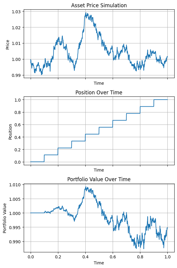
Here is a very simple simulation of what that would look like:
Analysis
We want to compare the return over period $T$ of the two strategies.
For the first one, lump sum, it is extremely straightforward. We simply have a position of $W = 1$ on an asset that has return distribution $N(\mu, \sigma)$ (We assume the time period is sufficietly short so that we can neglect 2nd order terms numerically). In that case, the return distribution of our strategy is simply $N(\mu, \sigma)$. That gives us a Sharpe ratio of $\frac{\mu}{\sigma}$.
Now, let’s delve into the DCA strategy.
If we denote by $\Delta_i$ the variation of asset price between time $t_{i-1}$ and $t_i$, we have the total variation of the asset price over period $T$ which is
\[\Delta := \Delta_1 + ... + \Delta_n\]Because the price of the asset (which we will denote by $X_t$) over period $T$ follows approximately an arithmetic Brownian motion (ABM) - again for sufficiently short $T$ - we have for all $i$:
\[\Delta_i \sim N(t_i \mu, \sqrt{t_i} \sigma) = N(\frac{\mu}{n}, \sigma \sqrt{\frac{1}{n}})\]Because $X_t$ is an ABM, we have $\Delta_i$ independent from one another.
The variation of the portfolio value during time interval $[t_{i-1}, t_i]$ is:
\[i w \Delta_i = \frac{i \Delta_i}{n} \sim N(\frac{i t_i \mu}{n}, \frac{i \sqrt{t_i} \sigma}{n}) = N(\frac{i \mu}{n^2}, \frac{i}{n} \sigma \sqrt{\frac{1}{n}})\]Therefore, if we write $w_i := \frac{i}{n}$ the exposure to the asset during time interval $[t_{i-1}, t_i]$, we have:
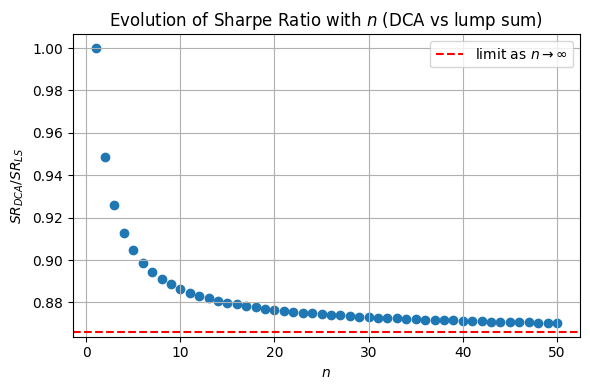
\[\Delta \sim N((w_1 t_1 + ... + w_n t_n) \mu, \sqrt{w_1^2 t_1 + ... + w_n^2 t_n} \sigma) = N((1 + ... + n) \frac{\mu}{n}, \sqrt{1 + ... + n^2} \frac{\sigma}{n^{3/2}})\] \[= N(\frac{n (n + 1) \mu}{2 n^2}, \sqrt{\frac{n (n + 1) (2n + 1)}{6n^3}} \sigma) = N(\frac{(n + 1) \mu}{2n}, \sqrt{\frac{(n + 1)(2n + 1)}{6 n^2}} \sigma)\]This is the most simple anayltical formula we can get for the distribution of returns. We can study the asymptotic properties as $n \rightarrow \infty$.
\[\Delta \sim N(\frac{(n + 1) \mu}{2n}, \sqrt{\frac{(n + 1)(2n + 1)}{6 n^2}} \sigma) \rightarrow N(\frac{\mu}{2}, \frac{\sigma}{\sqrt{3}})\]The Sharpe ratio for such a strategy is $\frac{\sqrt{3} \mu}{2 \sigma} < \frac{\mu}{\sigma}$. So a DCA with continuous allocation until the closure of the position underperforms the lump sum strategy in terms of SR, by a factor of $\frac{\sqrt{3}}{2} \approx 0.87$.
The maximum SR is reached for $n = 1$ which corresponds to the lump sum.
Conclusion
Using a very simple, yet powerful model we showed that DCA was suboptimal in terms of Sharpe ratio compared to lump sum.
However, one could argue that there are many types of DCA, and we don’t need to have a constant fraction of the target position that is invested (neither constant time intervals). For example, we could imagin investing variable fractions $(w_1, …, w_n)$ until we reach the target position, still on evenly spaced time intervals. This is just an optimization problem, that would be interesting to solve, but that will be for another post.