Introduction

This project was conducted when I was in my first year at Ecole Nationale Supérieure d’Arts et Métiers. One organization was present on the campus I was on (the Bordeaux one), named the NAASC (short for Nouvelle Aquitaine Academic Space Center) that regularly funded experimental rocketry projects. I knew a friend who was in contact with another student willing to do this kind of project, we contacted him and joined the team.

The team was pretty hefty - more than 30 people from what I remember, each from various engineering schools around the Bordeaux area, majoring in ME, EE & more. On top of that, there was this student we talked about before, that was sort of the designated project manager. This student, we will name him Jean-Pierre for privacy purposes, was rather autonomous and participated in a lot of design operations - this will play an important role for what comes next.

This big team was split into subdivisions of people from the same university. And each subdivision was responsible for (surprise) a subdivision of the bigger system that was the rocket.

To put things in context, that was not the first year this project had been occuring. Indeed, we could access to the database of technical files of previous years’ launches, helping us in the design process - although one could argue these repositories were (extremely) messy. And, thanks to these previous successes, we had the confidence of the NAASC to build a bigger rocket than previous years. In practice, this meant a bigger engine, i.e. one with more fuel, allowing us to reach higher altitudes. We’ll see later in the simulations, but the altitudes reached were expected to be ~1.7 km. The size of the full rocket was around 2 meters.

Anyway, our team - the Arts et Métiers team - was in charge of the design of the recovery system for this small rocket. For those unfamiliar with experimental rocketry, we call recovery system the parachute and its gear. It is critical for safety reasons: you do not want the rocket to just fall and crash on the ground after it reached apogee.

I just put it here, but generally speaking at Arts et Métiers, people are not big CS fans. However, I was kind of an outlier on this aspect so I got assigned to implementing the algorithm for the control of the recovery system.

This is a rather simple bang-bang control problem. The current control algorithm was pretty archaic - it consisted in a simple timer which delta was computed during simulation using a spreadsheet provided by NAASC, and an Arduino Nano would just send the signal to the step motor to open the trapdoor, releasing the parachute.

However, this solution did not adapt to the variability of the physical conditions during the flight. Imagin some wind perturbates the trajectory and the parachute triggers during ascension - this could set it on fire. Or also imagin it releasing too late. the rocket could have accumulated so much speed that (because frictions are proportional to $v^2$) the strings of the parachute would break.

For all the above reason, the natural upgrade was to go from a timer-based control to an apogee-detection control.

In principle, this is rather simple: you take the accelerometer data, integrate it twice, and see when the derivative is zero.

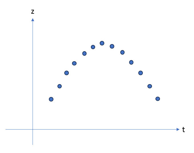
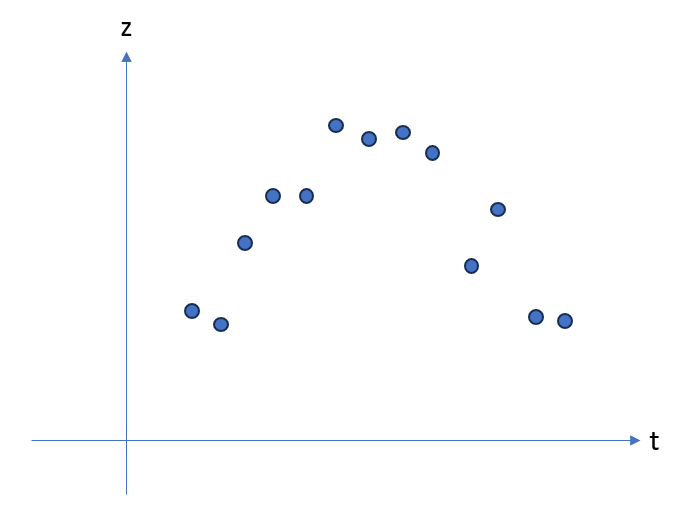
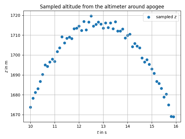
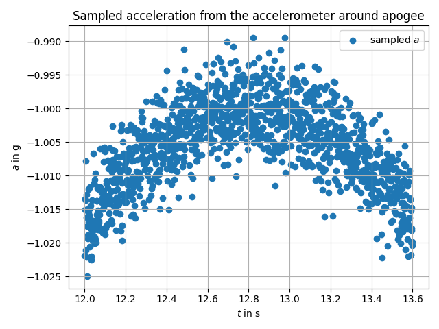
Except the derivative is never actually zero. Indeed, we have some important mechanical noise in the signal due to turbulences of the air flow around the rocket. So the trajectory data is not of the form of the first figure, but more of the one of second figure.

alt text — Clean altimeter data (ideal).

So, there was the clear need for filtering of that data. But I think this is enough for the introduction. In short: the problem is to build a precise apogee detection algorithm in order to achieve optimal timing for the deployment of the parachute, securing aerodynamic performances of the parachute.

Preliminary Data Generation

Before we even start the design process, it is important to have some actual data to work with. Unfortunately, the previous teams did not put their launch data on the repository, so we had to generate it.

We have two major data sources in our case:

One altimeter we could arbitrarily choose.
One accelerometer, same story.

So we had to get representative altitude data, as well as acceleration data. We did not use attitude data, which could arguably be a weakness in our approach since there is no guarantee the rocket will ascend perfectly vertically (we indeed know for sure it is not the case).

So, how do we generate some data for these two sensors? The most straightforward way is to build a simple model for the rocket’s dynamics. We will use the physical constants derived from our estimated components. We will then be able to numerically integrate the obtained set of ODEs, and add gaussian noise to our results to model mechanical noise.

Rocket Equation with Constant Gravity and Quadratic Friction

The Non-Ideal Rocket Equation (PDF download)

The above document provides all the mathematical details of deriving the differential system used for simulation. I will just give the main ideas here:

We use the conservation of total momentum in a similar fashion than when we derive the Tsiolkowsky equation.
Except this time we add quadratic friction as well as a constant gravity field - this is justified by the moderate altitudes of the rocket (you don’t feel zero gravity when you go hiking).

We end up with the following equation for speed:

\[\dot{v} = Q(t) v_e -\frac{\rho S C_d}{2 m(t)} v^2 - g\]

With $m(t) = m_0 - Q(t) t$ and:

\[Q(t) = \begin{cases} Q_0 \quad \text{for } t < T_p := \frac{m_0}{Q_0}\\ 0 \quad \text{otherwise} \end{cases}\]

With constants:

$v_e$ the ejection speed of the propellant in m/s.
$\rho$ the density of air in $kg/m^3$.
$S$ the right section of the rocket in m².
$g$ the gravity field at sea level in m/s².
$Q_0$ the mass flow rate of the engine in kg/s.

The state-space representation can be closed by adding $v = v$.

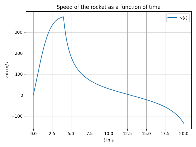
We can then perform numerical integration, here are the results (we plugged in typical values for the constants after looking at the technical documentation of the most usual components):

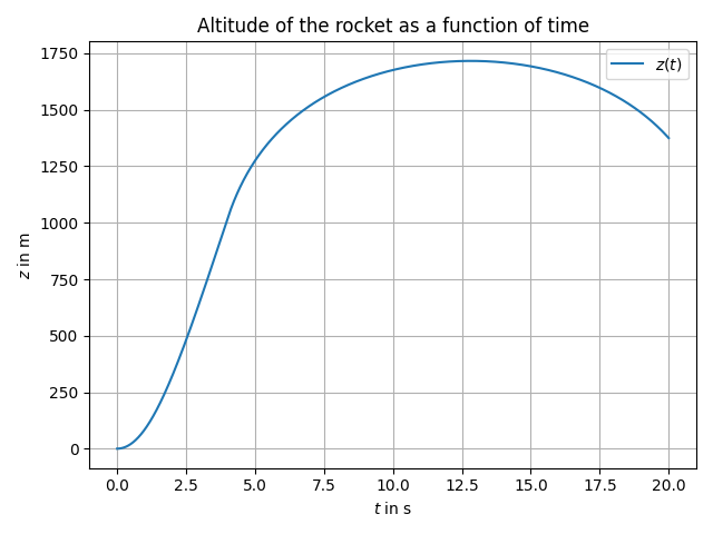
This was also the first time we had an estimate of the maximum altitude of the rocket: around 1.7 km.

Modelling Mechanical Noise and Sensor Measurement Uncertainty

To model mechanical noise and measurement uncertainty, we simply added some iid gaussian noise to our data, with variance scaled using the typical values from the technical documentation of the most common altimters and accelerometers. We also needed to estimate the amplitude of teh mechanical noise. All the values can be found on the GitHub repo (link at the top of the page).

So the data we will work with will look like this:

Design v1 - First Order LPF

The initial (naive) idea was to use a first order low-pass filter (LPF) with a chosen cut frequency. For those unfamiliar, a first order LPF is a filter that performs:

\[\hat{x}_{t+1} = \alpha x_t + (1 - \alpha) \hat{x}_t\]

where $\hat{x}_t$ is the estimated value of the signal (post filter) at time $t$, and $x_t$ its actual measurement. $\alpha$ is a constant between 0 an 1 and we have:

\[\alpha = \frac{T_e}{\tau_c + T_e}\]

where $\tau_c = \frac{1}{2 \pi f_c}$ is related to the cutoff frequency in Hz $f_c$, and $T_e$ is the sampling period (we have $1/T_e \approx 10 Hz$ for a commercial barometric altimeter, and $\approx 1 kHz$ for an accelerometer).

The good thing with that filter is that it is perfectly causal - it means that it can be used in real time since it does not require future data. However, there is a major flaw in this filter, that is shown in belows’s figures.

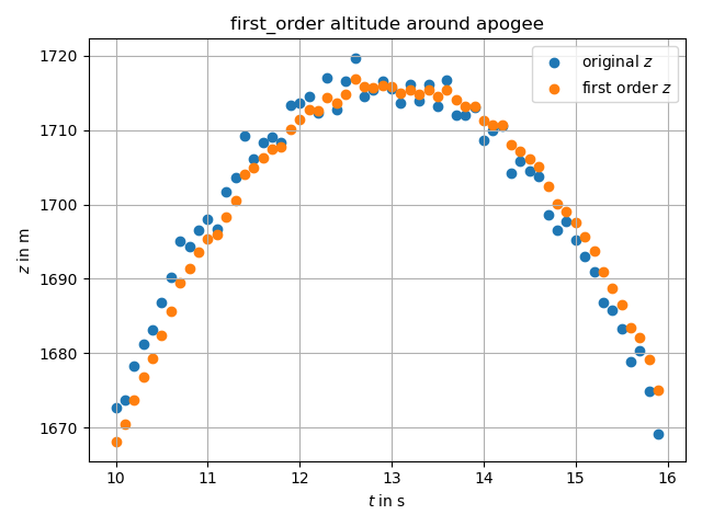
When we tuned the value of $f_c$ to cut more and more high frequency content from our signal, we observe some phase shift. The effect is even more pronounced as we decrease the value of the cutoff frequency. This is expected behavior, since the first order LPF is an integrator in the cutoff domain.

The bad thing is that filter is not suitable for our application. We have to trade frequency cutting against latency in apogee detection, which is not viable. We had to switch approaches.

Design v2 - Kalman Filter

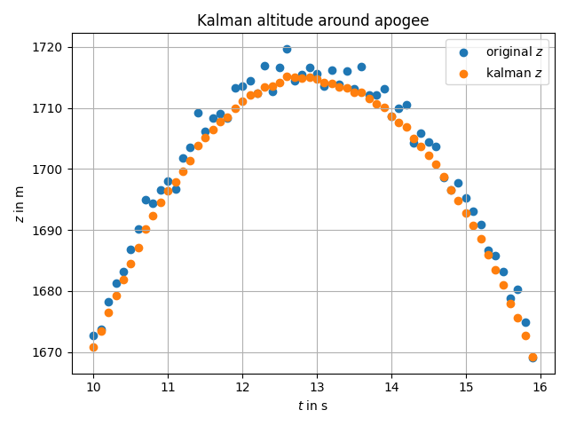
The Kalman filter is not exactly a filter like the 1st order LPF or a 4th order Butterworth filter. However, I like to think of it as a causal filter with zero phase shift. Indeed, no causal filter can achieve zero phase shift using only transformation of the data. So the price we have to pay in order to get this zero latency is we have to know a model for the dynamics of our rocket. Fortunately enough, we already established such a model in the Rocket Equation with Constant Gravity and Quadratic Friction section. We just have to put it in the correct form to apply the Kalman filter algorithm.

Implementation details can be found in the repo of the project, here are some plots of the effect of the Kalman filter on the noisy signal. Once again, we recall that this filter is causal.

Design v3 - Pure Data-Driven Approach

The solution of the Kalman filter is very elegant, and is probably the one we would end up using in the industry. However, it is still interesting to get a pure data driven approach that does not rely on a model of any kind. This is especially popular in modern robotics where practitioners are transitionaing away from classical physics-driven control to data-driven control using techniques such as Deep RL or JEPA.

In our case, we will use none of that fancy (yet very interesting) stuff, we will take a much simpler and naive approach: what if we could get a sort of 1st order Taylor expansion of the underlying signal? That is indeed the assumption we, as human, make when we look at anoisy signal: in order to get the next point we would just fit a straight line to the previous data points and take the intersection with that straight line for the estimate of the actual position (see figure below).

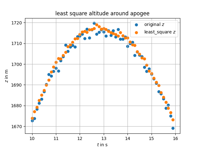
That is exactly what we implemented in code. We chose a fixed set of data points (optimized for computability using a Raspberry Pi, and taking into account the sampling frequency) before time $t$ and fit a linear regression to these data points to estimate the position at time $t+1$. This results in smoothing without the need of any form of model. However, our approach assumes:

High frequency (HF) content is not inherent to the underlying signal, and is clearly distinguishible from LF content.
The signal is continuous - although the Kalman filter also makes this assumption.

So, What Happened Next?

Unfortunately, this experimental rocketry project never finished. After finishing the apogee detection algorithm, I jumped to more hardware considerations (mostly getting the bill of materials for the recovery system, so choosing the right cables, making some electronics CAD, helping the actuators’ team…). But in the mean time, the team had to face massive departures due to internships, so much so that only about half of the people that were initially working on the project could continue it. Among the people that left the project, our project manager Jean-Pierre.

The moment was critical since we had to present the actual design to the NAASC so they could give us the fundings to buy and/or manufacture the different parts of the rocket. My friend tried to manage the project but the difficulties we had reaching out to Jean-Pierre to conduct knowledge transfer discouraged us and we ended up leaving the project too.

This is not a triumphant ending, it sucks given the amount of work we put in this. Yet, now I tell it, I recognize it as a great learning opportunity. My takeaway is that project management is key to the success of any project. Indeed, even when Jean-Pierre was still in the team, he worked mostly by himself for his parts of the rocket, and did not take the initiative to ease communication between the different subdivisions of the team, even with himself. So when he dropped the project, the knowledge transfer was impossible. This underlines the importance for a project manager to delegate work. Ideally, a project manager should never get involved in the actual work of the project, they should only command the different stakeholders - this is especially true as the team gets bigger.

If I tell this project even though I don’t have pretty pictures of a rocket launch, it is because it then had a great impact on the way I approached my future projects. I tried to learn from the mistakes we made, and made sure that every team I took part in had a designated leader, even if it meant me fulfilling this role.

Besides that, it was also extremely stimulating from a scientific and engineering point of view. I had the occasion to collaborate with extremely talented people and it was one of the first times I used knowledge I had learned in academia to address a real-world challenge. If I want to be even more specific: the understanding I got of Kalman filters as zero-phase-shift filters is a precious idea that greatly helped me understand when to use them.

Thanks for reading this project presentation, I tried to make it the most digest by introducing some story-telling. This might differ from what you might be used to when reading portfolios, where people focus on efficiency and results. Do not hesitate to email me if you like it or if you don’t.

Have a nice day!